Biases in logistic regression - it is not about N (Part 1)
Here is a short script I used to run often:
from sklearn.linear_model import LogisticRegression
model = LogisticRegression()
model.fit(X, y)
But there could be a problem in this naive implemtation of logistic regressions. In this post, we will talk about what it is.
Logistic regression + Rare events data
Logistic regression is probably the most widely used model (or the first approach one would try) for binary classification problems1. A very simple form and easy to fit. The typical way to estimate it is by maximizing the log likelihood, which is pretty cheap2.
Now, here is a phrase you might have heard from some STATS101, about the maximum likelihood estimation:
“Maximum likelihood estimators (MLE) are asymptotically unbiased.”
OK, it’s good to know, but in practice, who cares? When your data has, say, 1000000 rows, would you really worry about the biasedness of your estimators?
Well, it depends on the problems, and I guess usually you should be fine as long as you have a decently large number of samples. This is simply because the rate of convergence of MLE is in the order of $N$.
However, if you’re dealing with rare events data, large $N$ may not be enough.
This is because the “rareness” (of events) plays a role, too, for the convergence rate of MLE. More precisely, it is not specifically about “rareness”, but more about the actual number of events recorded in your data (we’ll see this later)
Still not super clear, so let’s check it out directly with numbers.
Simulations
Here is a toy experiment with synthetic data:
- Pick sample size: $N \ \ (=10^6)$
- Pick true parameters: $\beta_0$ and $\beta_1$.
- Generate
X: $x_i$~ unif[0,1]($i=1, …, N$) - Generate
y: $y_i$ with the probability of events for each $x_i$: \(P(y_i=1 | x_i, \beta_0, \beta_1) = \cfrac{1}{1 + e^{-\beta_0-\beta_1 x}}\) - Run logistic regression estimation with
(X,y)to get the MLE: $\widehat{\beta_0}$ and $\widehat{\beta_1}$. - Compare ($\widehat{\beta_0}$ , $\widehat{\beta_1}$) with ($\beta_0$ , $\beta_1$).
Here are the results from a few different cases.

| Case | (average) Probability of Events3 | $\beta_0$ | $\widehat\beta_0$ | $\beta_1$ | $\widehat\beta_1$ |
|---|---|---|---|---|---|
| #1 | 0.867663 | 1 | 0.996953 | 2 | 2.005827 |
| #2 | 0.098371 | -1 | -1.005705 | -3 | -2.993025 |
| #3 | 0.003017 | -4 | 4.032847 | -6 | -5.952327 |
| #4 | 0.000101 | -7 | -7.117254 | -9 | -7.933081 |
| #5 | 0.000034 | -8 | -8.168674 | -10 | -8.862332 |
Note that ($\widehat{\beta_0}$ , $\widehat{\beta_1}$) are fairly close to ($\beta_0$ , $\beta_1$) in #1, #2, and #3, but not in #4 and #5. That is, when the probability of events is very small, the MLEs are biased. We used the same $N(=10^6)$ in all cases, so $N$ shouldn’t be solely blamed for the biases.
Then, is it all about $P$, the probability of events?
More Simulations
In order to get a better sense of what is going on, let’s draw more random numbers along with various configurations.
- Consider the following combinations of $N$ and $P$:
- $N$: 10000, 50000, 100000, 500000, 1000000
- $P$ (probability of events): 50%, 11.2%, 5.73%, 1.17%, 0.59%, 0.12%
- In each pair of ($N,P$), repeat the above toy experiment $M$ times, to have $M$ ensembles of MLEs: $\widehat\beta^{(m)}$ ($m=1, …, M$).
- Compare $\widehat\beta^{(m)}$ with the true parameter ($\beta$) by the following error metric4: \(\textsf{Mean Absolute Relative Error (MARE)}=\displaystyle \sum_{m=1}^M\cfrac{|\widehat\beta^{(m)}-\beta|}{|\beta|}\)
See below for the results. Clearly, some trends are observed:
- Given $N$, the error increases as $P$ decreases.
- Given $P$, the error levels are higher for smaller $N$.

What is more interesting is the next one.
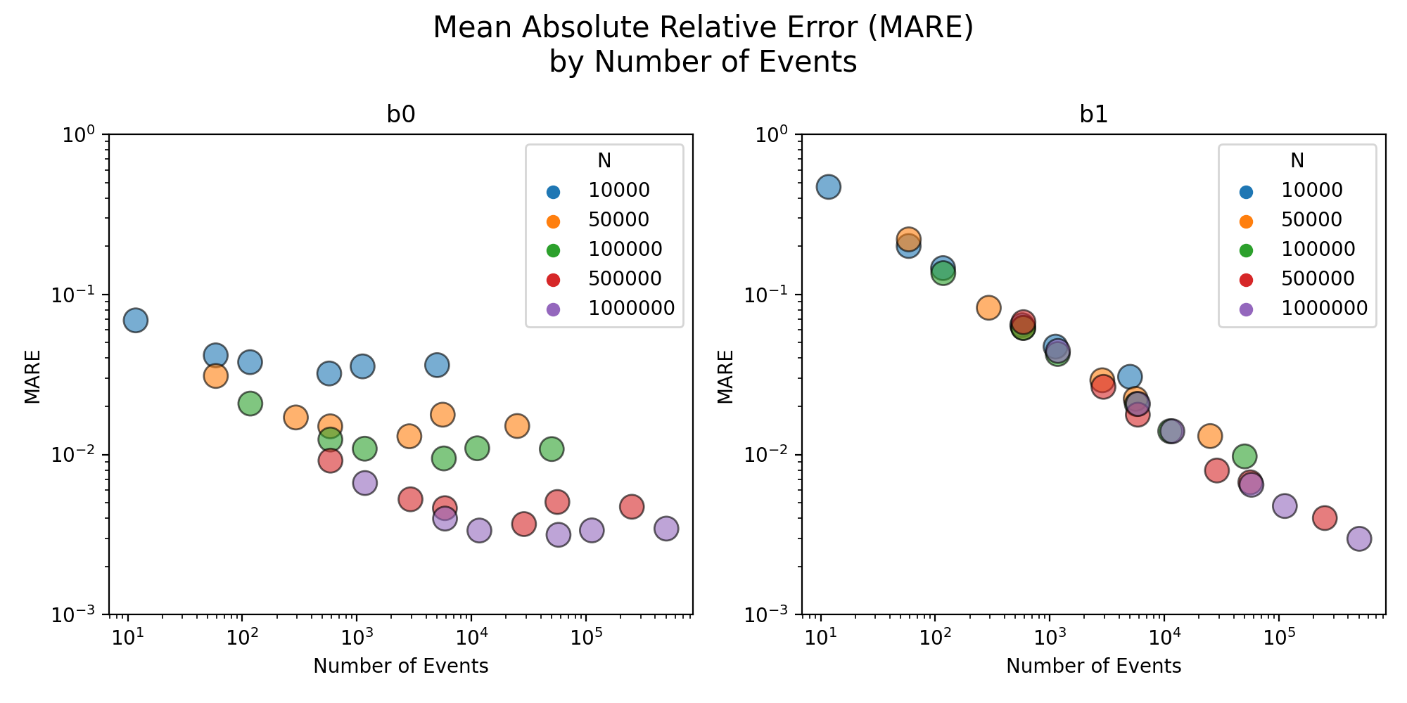
This shows the error of the MLE $\widehat\beta_1$ with respect to the number of events. Take a look at the right plot ($\beta_1$) - all the dots are on the same line5. That is, regardless of $N$, it is the actual number of events (call it $N_{events}$) that matters.
So what?
So, $N_{events}$, not $N$, determines the biases.
You’d be better to have many instances of events in your data, no matter how many rows it has. From a practical point of view, this is not something pleasant to realize. Yeah, we hear the hype of big data everyday, but many real problems are not big data problems. Think about clinical data collected from patients. Collecting each patient’s medical records is usually very tedious or sometimes impossible. So even if you collect such data from a handful of medical institutions, $N$ might be merely several hundreds or thousands at most. What about $N_{events}$ (e.g., number of diagnosed patients)? It should be even much smaller (and we saw from the above simulations that if $N_{events}$ is 100, the relative bias from logistic regression is about 15%, for example).
In many cases where we use logistic regressions for modeling, $N_{events}$ is usually quite small, either because $N$ itself is not large or because $N$ is large but $P$ is very small. Then the biases are already there, from the beginning6.
I will stop here for now. In a later post, I will continue the discussion and talk about remedies for the biases.
Codes: https://github.com/uriyeobi/bias_in_logistic_regression
Notes
-
To name a few examples of binary signals - passengers on the Titanic, credit card fraud, loan defaults, or breast cancer. ↩
-
via Newton’s method, since the log likelihood function in this case is convex. Nowadays, it is just a one liner with available packages - statsmodel, sklearn , or glm. ↩
-
Since $x_i$
~ unif[0,1], the mean of probability of events can be calculated from a direct integration: $E\Big[P(y=1;\beta_0, \beta_1)\Big] =\displaystyle\int_0^1 \cfrac{1}{1 + e^{-\beta_0-\beta_1 x}}dx=\Bigg[\cfrac{\log\big[e^{\beta_0+\beta_1x}+1\big]}{\beta_1}\Bigg]_{x=0}^{x=1}$. For example, with $\beta_0=-1$ and $\beta_1=-3$, this is $\approx 0.098371$. ↩ -
Other metrics could be used, but the big picture wouldn’t change. ↩
-
For $\beta_0$, the behavior is similar, but there are some plateau regions. ↩
-
When I was working in a bank, there was a struggling moment when our forecast model (part of which involves logistic regressions) couldn’t capture certain corporate credit events properly. This post is partly motivated from that experience. ↩